2 Random walk on an Undirected Graph
The state distribution after a random walk on a graph can be found using the transition probability matrix.
Let's examine the following graph.
g1 = graph.formula(1 - 2, 1 - 3, 1 - 4, 2 - 3)
plot(g1)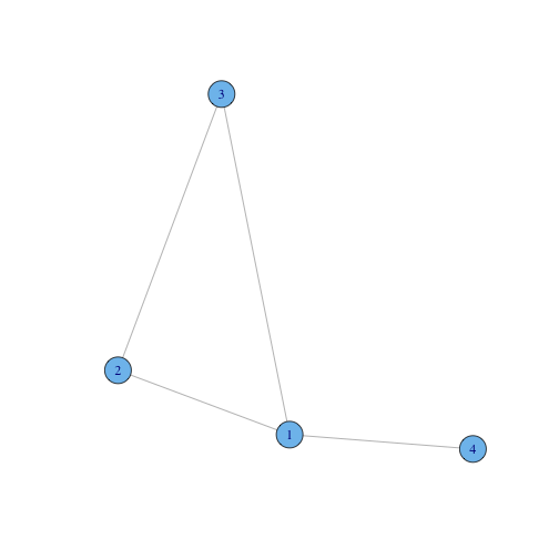
The graph g1
We can obtain the adjacency matrix of g1:
A = get.adjacency(g1)
print(A)
## 4 x 4 sparse Matrix of class "dgCMatrix"
## 1 2 3 4
## 1 . 1 1 1
## 2 1 . 1 .
## 3 1 1 . .
## 4 1 . . .2.1 Transition probability matrix
The transition probability matrix is the adjacency matrix, with all columns scaled so they sum to 1.
To create the transition probability matrix, we will write the function adjacency.to.probability that takes the adjacency matrix A and divides each column by its sum.
adjacency.to.probability = function(A) {
    cols = ncol(A)
    for (a in 1:cols) {
        A[, a] = normalise(A[, a])
    }
    return(A)
}
This function uses the function normalise on each column, but this function does not exist yet.
Write the function
normalisethat takes a vectorxand returns the vectorxdivided by its sum.
Now compute the transition probability matrix T:
T = adjacency.to.probability(A)Examine T to make sure that the columns sum to 1.
2.2 Stationary distribution using the Power Method
We can now use T to take a step in a random walk on the graph g1.
We will start our random walk on vertex 1, which means the probability of being on vertex 1 is 1, and the probability of being on all other vertices is 0. Therefore, our initial state is:
p = c(1, 0, 0, 0)To take a random step, we multiply the matrix T with the state p. Matrix multiplication in R is performed using the operator %*%:
p = T %*% p
print(p)
## 4 x 1 Matrix of class "dgeMatrix"
## [,1]
## 1 0.0000
## 2 0.3333
## 3 0.3333
## 4 0.3333Does the new state distribution
pmake sense?
To take another step, multiply the new state distribution by T:
p = T %*% p
print(p)
## 4 x 1 Matrix of class "dgeMatrix"
## [,1]
## 1 0.6667
## 2 0.1667
## 3 0.1667
## 4 0.0000And another:
p = T %*% p
print(p)
## 4 x 1 Matrix of class "dgeMatrix"
## [,1]
## 1 0.1667
## 2 0.3056
## 3 0.3056
## 4 0.2222If we repeat this process, we find that the state distribution starts to converge. The distribution it converges to is the stationary distribution.
Rather than running the code manually, we can write a while loop that repetitively runs the code, while there is a change in the state distribution.
Let's write a function that contains the while loop, called stationary.distribution.
stationary.distribution = function(T) {
    # first create the initial state distribution
    n = ncol(T)
    p = rep(0, n)
    p[1] = 1

    # now take a random walk until the state distribution reaches the
    # stationary distribution.
    p.old = rep(0, n)
    while (difference(p, p.old) > 1e-06) {
        p.old = p
        p = T %*% p.old
    }
    return(p)
}
The above function requires us to write the missing function difference, that returns the Euclidean distance between two vectors.
Write the function
difference, that returns the Euclidean distance between two vectors.
Now compute the stationary distribution:
p = stationary.distribution(T)
print(p)
## 4 x 1 Matrix of class "dgeMatrix"
## [,1]
## 1 0.375
## 2 0.250
## 3 0.250
## 4 0.125The stationary distribution should satisfy the equation: \[ \vec{p} = T\vec{p} \]
Check if the computed stationary distribution satisfies the stationary distribution equation.
2.3 Stationary distribution using the Eigenvalue Decomposition
We can also compute the stationary distribution using the eigenvalue decomposition.
Remember that and eigenvalue \(\lambda\), eigenvector \(\vec{v}\) pair of the square matrix \(A\) satisfy the equation: \[ \lambda\vec{v} = A\vec{v} \] In our case, we want the vector \(\vec{p}\) that satisfies: \[ \vec{p} = T\vec{p} \] Therefore, \(\vec{p}\) is an eigenvector of \(T\), with eigenvalue \(1\).
We can compute the eigenvalue decomposition in R using the function eigen:
e = eigen(T)
print(e)
## $values
## [1] 1.0000 -0.7287 -0.5000 0.2287
##
## $vectors
## [,1] [,2] [,3] [,4]
## [1,] -0.7071 0.8586 -4.441e-16 -0.4034
## [2,] -0.4714 -0.2329 -7.071e-01 0.4957
## [3,] -0.4714 -0.2329 7.071e-01 0.4957
## [4,] -0.2357 -0.3928 2.875e-16 -0.5880The eigenvalue decomposition has found four eigenvalues and four associated eigenvectors (the columns of e$vectors). We want the eigenvector associated to the eigenvalue of 1. We can see that the eigenvalue equal to 1 is the first in the list of eigenvalues, so we want the first eigenvector.
p = e$vectors[, 1]
print(p)
## [1] -0.7071 -0.4714 -0.4714 -0.2357Does the value of
plook like the stationary distribution?
The stationary distribution must sum to 1 (for it to be a distribution). Therefore we normalise the chosen eigenvector to obtain the stationary distribution of graph g1. We wrote the function to perform this normalisation, so we can use it again.
p = normalise(e$vectors[, 1])Examine
pto make sure it is the stationary distribution.
Create a new graph
g2and compute its stationary distribution using the Power Method and the Eigenvalue decomposition.