For this lab, we will be using the igraph
package. Install the package before beginning the lab:
install.packages("igraph")
If the package does not download due to the UWS proxy server, see Lab 5 for further information on installing packages.
Once installed. Load the library:
library("igraph")
To create a graph, we can use the formula interface or provide an adjacency matrix.
We can create a graph by providing the graph.formula
function with the set of vertices, and how they are connected (edges). For example:
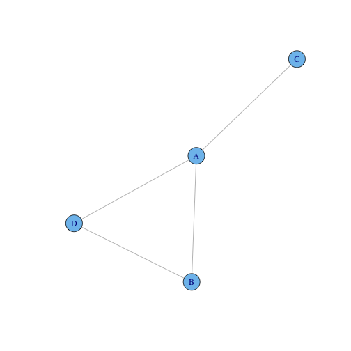
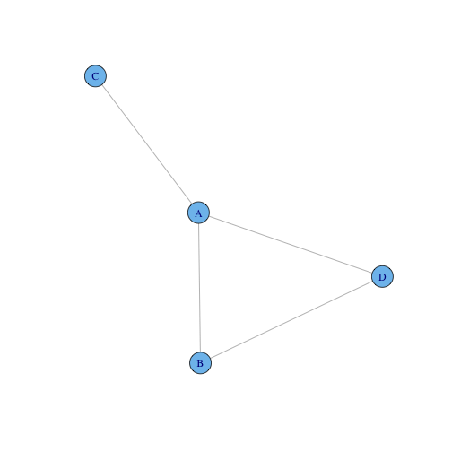
g1 = graph.formula(A - B, A - C, A - D, B - D)
To view the graph, we can print out the graph variable g1
:
print(g1)
## IGRAPH UN-- 4 4 --
## + attr: name (v/c)
To view the vertices of the graph, use the function V
:
V(g1)
## Vertex sequence:
## [1] "A" "B" "C" "D"
To view the edges, use the function E
:
E(g1)
## Edge sequence:
##
## [1] B -- A
## [2] C -- A
## [3] D -- A
## [4] D -- B
To visualise the graph, plot it:
plot(g1)
To create a graph from an adjacency matrix, we must first create the matrix. An adjacency matrix \(A\) contains \(N\) rows and columns, where \(N\) is the number of vertices. The element \(a_{i,j}\) of \(A\) is the element from the \(i\)th row and the \(j\)th column. If there is an edge between the \(i\)th vertex and \(j\)th vertex, then \(a_{i,j} = 1\). If there is no edge, then \(a_{i,j} = 0\).
We can first make a \(4\times 4\) matrix, containing all zeros:
A = matrix(0, 4, 4)
Then add the edges by allocating ones. We will make the same graph shown above in g1
. We want to connect the first vertex to the second, third and fourth vertices:
A[1, c(2, 3, 4)] = 1
We also want to connect the second vertex to the first and fourth:
A[2, c(1, 4)] = 1
We connect the thrid vertex to the first:
A[3, 1] = 1
And connect the fourth vertex to the first and second:
A[4, c(1, 2)] = 1
Giving us:
print(A)
## [,1] [,2] [,3] [,4]
## [1,] 0 1 1 1
## [2,] 1 0 0 1
## [3,] 1 0 0 0
## [4,] 1 1 0 0
Notice that the matrix is symmetric. Adjacency matrices for undirected graphs are always symmetric, showing that the edges can be followed from either direction.
We create the matrix with:
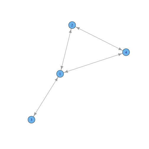
g2 = graph.adjacency(A)
and visualise it:
plot(g2)
Notice that the edges in the plot of g2
have arrows, implying that it is a directed graph. Examine the help page of the function graph.adjacency
and work out how to make the graph undirected.
We can also create a graph using an edge list. An edge list is an \(M\times 2\) matrix, containing \(M\) edges. Each row of the edge list provide the start and end vertices. For example:
el = matrix(c("A", "A", "A", "B", "B", "C", "D", "D"), 4, 2)
print(el)
## [,1] [,2]
## [1,] "A" "B"
## [2,] "A" "C"
## [3,] "A" "D"
## [4,] "B" "D"
We then create the graph:
g4 = graph.edgelist(el, directed = FALSE)
plot(g4)
We saw in the lecture that we are able to create an Erdős-Renyi Graph once given the parameters \(n\) (the number of vertices) and \(p\) (the probability of an edge appearing).
To create and Erdős-Renyi Graph:
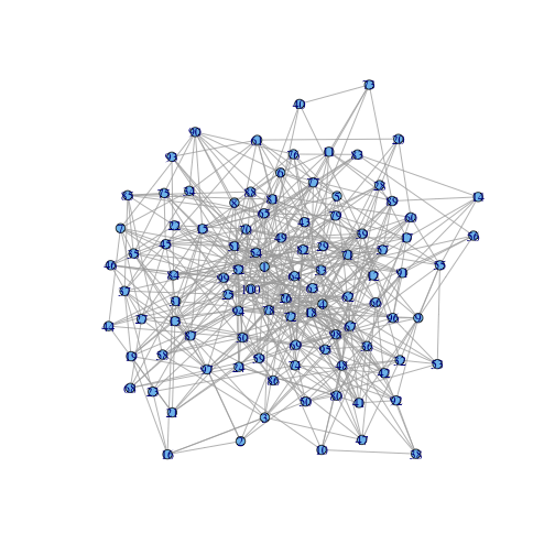
g.er = erdos.renyi.game(n = 100, p = 0.1)
plot(g.er, vertex.size = 5)
In the plot command, we reduced the vertex size so we can see the edges more clearly. Run the plot command without vertex.size = 5
to see the difference.
To create a Barabási–Albert Graph, we must provide \(n\) (the number of vertices). We can also provide the \(k\) (the power) and \(m\) (the number of edges to add to each new vertex).
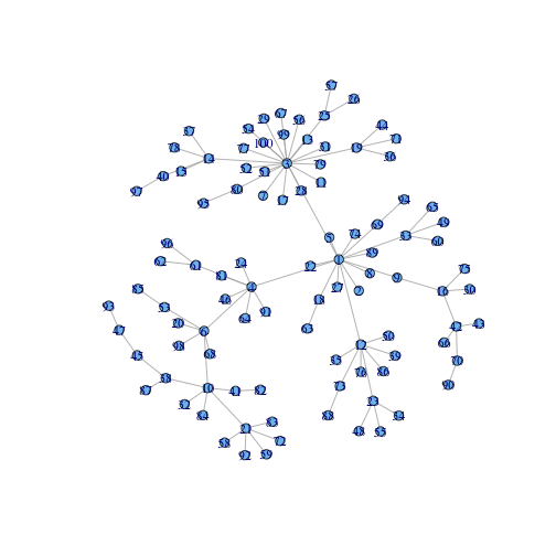
g.ba = barabasi.game(n = 100, directed = FALSE)
plot(g.ba, vertex.size = 5)
In this section, we will examine some of the functions that that available for us to examine properties of graphs.
By visually examining the two graphs above, which looks denser? Use the function graph.density
to compute the density of each graph and compare the results to your guess.
The diameter is the longest shortest path. Which of the two graphs do you expect to have the largest diameter? Use the function diameter
to compute the diameter of each graph.
What do you expect the degree distribution of each graph to look like? We can compute the degree of each vertex using the function degree
. We can also compute the degree distribution of the graph using the function degree.distribution
. Use the help
pages to understand the output.
Which vertex is most central according to Degree Centrality?
We defined the closeness centrality of a vertex \(v\) as the sum of the distance from \(v\) to all other vertices. To compute the closeness of each vertex, we use:
closeness(g.ba)
## [1] 0.003788 0.002762 0.003333 0.003311 0.002762 0.002793 0.002513
## [8] 0.002762 0.002890 0.002347 0.002513 0.002941 0.002513 0.002577
## [15] 0.002058 0.002326 0.002513 0.002778 0.002551 0.002193 0.001946
## [22] 0.002762 0.002315 0.002500 0.002538 0.002033 0.002762 0.002513
## [29] 0.002513 0.001894 0.002513 0.001908 0.002809 0.001887 0.002283
## [36] 0.002041 0.002058 0.001938 0.002283 0.002066 0.001916 0.001923
## [43] 0.001618 0.002041 0.001639 0.002500 0.001416 0.001887 0.002203
## [50] 0.002283 0.002513 0.002513 0.002203 0.002513 0.001887 0.002513
## [57] 0.002033 0.001634 0.001634 0.002203 0.002525 0.002024 0.002183
## [64] 0.002500 0.002203 0.001618 0.002513 0.002193 0.002778 0.001623
## [71] 0.002041 0.001634 0.002294 0.002762 0.001894 0.002283 0.002513
## [78] 0.002058 0.002513 0.002525 0.002500 0.001613 0.001634 0.001908
## [85] 0.001812 0.002283 0.001629 0.001873 0.002762 0.001401 0.002500
## [92] 0.001634 0.001244 0.002183 0.002024 0.002024 0.001718 0.002193
## [99] 0.002513 0.002513
This does not look right. The sum of differences should be an integer, but the R output is a set of real values.
Read the R help page for closeness
to find what R is computing. Then work out which of the vertices is the most central with respect to closeness centrality.
Betweenness centrality measures how often a vertex is used in shortest paths. We can compute betweenness using:
betweenness(g.er)
## [1] 171.33 28.29 48.91 74.90 48.95 57.37 41.30 36.59 63.63 20.07
## [11] 44.09 40.90 63.85 23.21 81.56 26.37 39.32 122.25 42.47 12.23
## [21] 23.68 27.77 21.35 55.03 47.72 173.35 36.42 27.46 84.79 114.21
## [31] 71.06 70.04 116.84 32.07 43.49 58.11 58.96 12.69 109.86 12.58
## [41] 40.13 55.89 61.97 18.53 66.74 25.08 19.68 81.12 61.62 42.52
## [51] 159.20 163.17 12.82 87.75 54.75 13.84 54.30 23.70 51.59 40.95
## [61] 59.32 65.92 106.04 92.58 107.34 95.37 121.86 16.12 124.45 113.40
## [71] 56.43 89.08 16.42 35.52 34.97 38.95 56.50 125.17 77.38 50.25
## [81] 86.64 77.95 39.86 61.29 36.61 28.60 66.14 34.50 61.11 47.45
## [91] 56.96 36.04 10.90 116.02 69.48 55.12 118.41 83.14 83.59 161.71
Is the centre the same for all three centrality measures? Examine this for the Erdős-Renyi graph and Barabási–Albert graph.
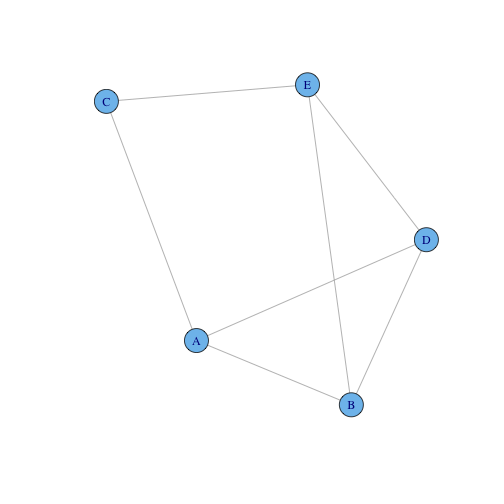
Using the following graph:
g3 = graph.formula(A - B, A - C, A - D, B - D, B - E, E - D, C - E)
plot(g3)
Calculate the:
using the methods shown in the lecture. Then check your answer using the R functions.
We will now access Twitter to obtain a graph constructed from a seed user.
Load the twitteR library:
library("twitteR")
## Loading required package: ROAuth
## Loading required package: RCurl
## Loading required package: methods
## Loading required package: bitops
## Loading required package: digest
## Loading required package: rjson
and register your application with Twitter using the process from Lab 5
Each twitter user has a set of friends and a set of followers:
Therefore, a user can choose their friends, but cannot choose their followers. There are many users of Twitter, we want to find the interesting ones. Interesting users usually have many followers (because they are interesting). So when obtaining information about users on Twitter, we should note:
Using twitteR
, we can download user information when given a screen name or ID. Let's examine Wil Wheaton:
user = getUser("wilw")
The variable user
is now a twitteR
object, which we can use as a seed for our graph.
To examine all of the details for Wil Wheaton, convert the twitteR object into a data frame:
user$toDataFrame()
The above function provides information such as the number of friends, the number of followers, if the account is protected and verified and the owner's name and id. Wil Wheaton is a popular person, so he must have popular friends. From the output of user$toDataFrame()
identify how many friends Wil Wheaton has.
We now want to download the list of Wil Wheaton's friends. Since he has a large number of friends, we download the first 100.
friends = user$getFriends(100)
The above function gets the friends of user
; since user
contains Wil Wheaton's details, the function returns a list of his friends. The list of friends is a list of twitteR
objects, so friends[[1]]
is the same data type as user
.
We now have the details of 100 of Wil Wheaton's friends. Examine the information of the first friend:
friends[[1]]$toDataFrame()
We can find which friends are the most popular by examining their follower count. Here we examine the follower count of the first friend:
friends[[1]]$getFollowersCount()
To examine the follower count of all friends:
follower.count = c()
for (a in c(1:length(friends))) {
follower.count[a] = friends[[a]]$getFollowersCount()
}
Let's make this a function for convenience:
count.followers = function(friends) {
follower.count = c()
for (a in c(1:length(friends))) {
follower.count[a] = friends[[a]]$getFollowersCount()
}
return(follower.count)
}
Find the 10 friends that have the most followers. What are their names? Note the function sort
will sort the vector of follower counts. The function order
will sort, but provide the position of the sort. So to find the top 10, we use order
with decreasing=TRUE
and choose the first ten values, giving us the positions of the top 10.
Some Twitter accounts are protected, meaning that we can't read them unless we are a follower. We can detect if the first friend account is protected using:
friends[[1]]$getProtected()
Write a for
loop to check if any of the friend accounts are protected and store the TRUE
/FALSE
values in the variable protected.status
.
Once we have the vector protected.status
, we can extract the unprotected friends of Wil Wheaton:
unprotected.friends = friends[!protected.status]
This will select the positions that are FALSE (the exclamation mark ! changes FALSE to TRUE and TRUE to FALSE).
Using the function count.followers
find the 10 unprotected friends with the most followers and store them in top.unprotected.friends
.
Now that we have the list of top 10 unprotected friends, we can use this to download the friends' friends. Lets create a place to store the friends of friends.
more.friends = list()
We can download a list of 100 friends of the first friend of Wil Wheaton using:
more.friends[[1]] = top.unprotected.friends[[1]]$getFriends(100)
Write a for
loop to download 100 friends from the 10 most popular friends of Wil Wheaton and store them in more.friends
.
Now we have Wil Wheaton, 100 of Wil Wheaton's friends, and 100 of 10 of Wil Wheaton's most popular friends.
We can create a graph by constructing an edge list (who links to who). We know Wil Wheaton links to all of his 100 friends, so the edge list will contain 100 rows beginning with Wil Wheaton and ending with the friend of Wil Wheaton. First we must get the names of all of Wil Wheaton's friends.
First we allocate a variable to contain the names:
friend.names = c()
We can get the first name using:
friend.names[1] = friends[[1]]$getScreenName()
Write a for
loop to store all 100 screen names in the variable friend.names
.
We can now build the edge list using:
wil = rep(user$getScreenName(), length(friends)) # repeat Wil Wheaton's user name 100 times
el = cbind(wil, friend.names) # bind the columns to create a matrix
We need to do the same for Wil Wheaton's 10 most popular friends. To simplify the process, we should write a function.
Using what you have done above, write the function:
user.to.edgelist <- function(user, friends) {
# create the list of friend screen names
friend.names = c()
for (a in c(1:length(friends))) {
# enter missing code
}
user.name = rep(user$getScreenName(), length(friends)) # repeat user's name
el = cbind(user.name, friend.names) # bind the columns to create a matrix
return(el)
}
We can use the created function user.to.edgelist
to create the edge list for Wil Wheaton:
el.wil = user.to.edgelist(user, friends)
We can also build the edge list for the top 10 friends using a loop:
for (a in c(1:length(more.friends))) {
el.friend = user.to.edgelist(top.unprotected.friends[[a]], more.friends[[a]])
el.wil = rbind(el.wil, el.friend) # append the new edge list to the old one.
}
Now that we have the edge list, we can create the graph:
g = graph.edgelist(el.wil)
Let's plot the graph. Since there are many vertices, we will reduce the vertex size and use a spacial plot layout:
plot(g, layout = layout.fruchterman.reingold, vertex.size = 5)
This graph contains many vertices that we did not examine. To remove these, let's only keep the vertices with degree (in or out) greater than 1.
g2 = subgraph(g, which(degree(g, mode = "all") > 1))
This graph is now easier to visualise:
plot(g2, layout = layout.fruchterman.reingold, vertex.size = 5)
Who is at the centre of the graph? Use the centrality measures to examine this.
Examine the graph density. Is it sparse or dense?
Examine the degree distribution. Is this graph more similar to an Erdős-Renyi graph or a Barabási–Albert graph?